Rudy Deighton

  • Home
  • Inleiding
  • De Toekomst
  • Marketing Platform
    • Delta Media Strategie Modules
    • Online Marketing
    • Delta Social Media
    • Delta Media Service
    • Delta media Platform
    • Delta Marketing Platform
    • Online business marketing
    • Online Business
      • Worth for free now
      • Work from Home 2020
      • Gadgets
      • All about Windows
      • about Whatsapp
      • Whats the
      • About websites
      • New Ways
      • New Way of Watching
      • Virtual
      • Website
      • All about Video
      • How to Use
      • YouTube Info
      • All about Twitter
      • The Best of
      • About Apps
      • Google News
      • For Free
      • About This
      • Need More
      • Why should you
      • Iphone news
      • Interesting News
      • About Amazone
      • Some tips
      • About Netflix
      • All about Music
      • About Facebook
  • Luxury Platform
    • The Indulgence Business site
    • The Luxury Web site
    • The Ultimate Indulgence
    • The Indulgence Site
    • The Ultimate Luxury Information site
    • Online luxury
  • Projecten
    • Global Diamond Security
    • Aqualith Project
    • Delta Online Projects
    • Delta Media
    • Delta Media Projects
    • Crypto info
      • What is Cryptocurrency
      • Delta Media ICO systeem
      • Cryptocurrency Information
      • About miners
      • Best Bitcoin Bokers
      • Overview Cryptocurrency
      • BLOCKCHAIN WEB PLATFORM
      • Delta Media ICO Cryptocurrency
      • Bitcoin Ticker
      • ICO and Cryptocurrency modules
      • Cryptocurrency, Blockchain, Bitcoin modules
      • Delta Buy & Sale Token
      • Buy and sell digital currency module
      • ico – Crypto BlockChain Parallax module
      • Exchange Cryptocurrency module
  • Nieuws Platform
    • RegioTV Nieuws
    • Regionaal Nieuws Platform
    • Nieuws Regio’s Tiel
    • RegioTV Buren
    • RegioTV Neder-Betuwe
    • Regionaal Nieuws Tiel
    • Micro Locals Nieuws
    • Micro Locals project
    • Lokale CSM systeem
    • RegioTV nieuws
    • Politiek Nederland
    • Politiek Gelderland
    • Politiek Tiel
    • Regio Nieuwsberichten Tiel
    • Regionaal nieuws
    • Regionaal video nieuws
    • RegioTV Nieuws & info
    • Regio Nieuws
    • Online video nieuws
    • Online Nieuws
    • Nieuws online RegioTV
    • Regionale content video
  • Promotion
  • Delta Media
    • Delta Media
    • Adverteren grote fraude
    • Menu POS
    • Delta Global Security
    • Delta Evenementen
    • LinkedIn
    • Facebook
    • Facebook Group
    • Twitter
    • Terms & Policy
    • Contact
    • .
  • Ads prices
    • Online Blog promotion price
    • Online web sites prices
    • Global Promotion Platform
  • Home
  • Delta Media News
  • How to Use Conditional Formatting in Google Sheets
January 24, 2021

How to Use Conditional Formatting in Google Sheets

How to Use Conditional Formatting in Google Sheets

by rudy deighton / Sunday, 10 January 2021 / Published in Delta Media News

Conditional formatting is when you automatically format the styling of cells in your spreadsheet based on the data in each cell. Google Sheets lets you use conditional formatting to apply different fonts, fill colors, and other styles, making your spreadsheets instantly easier to read.

All you need to do to use conditional formatting is create some rules for your spreadsheet to follow. Below, we’ll show you how to create those conditional formatting rules with Google Sheets.

When to Use Conditional Formatting

You can use conditional formatting for pretty much any reason that you might typically format a spreadsheet. The main advantage is to save yourself time and ensure consistency, but conditional formatting also encourages you to think about the setup and styling of your spreadsheet in advance.

You could use conditional formatting to differentiate between types of data in a set, grouping together employees by their department, for example. Or you could also use it to draw attention to problematic values, such as a negative profit. On occasion, it may also be useful to downplay obsolete records, such as activities with a date in the past.

Related: Google Spreadsheet Tricks That Are Easy to Learn and Remember

How to Create Conditional Formatting in Google Sheets

Perhaps the best way to demonstrate conditional formatting is with a simple example. Start with a new spreadsheet, and follow the steps below:

  1. Enter some example values in a few rows.
    An example spreadsheet showing a column of 7 values between 1 and 3

  2. Highlight the range of cells that you want to be eligible for conditional formatting.
  3. From the Format menu, choose Conditional formatting.
    A Google Sheet showing the Format menu with the Conditional formatting item selected

  4. Change the Format cells if… dropdown to Is equal to.
  5. Enter one of your example values in the Value or formula box.
  6. Choose the formatting you want to add, such as a fill color.
    Google Sheets conditional formatting with a fill color

  7. Click Add another rule.
  8. Replace the previous value with a different one from your spreadsheet and select a different format or color for this value.
  9. Repeat the previous two steps for more values, using different formatting each time.
  10. Once finished, click the Done button to see a list of the rules you’ve created.
    Google Sheets conditional formatting example showing 3 rules highlighting several rows in different colors

Types of Condition That Google Sheets Supports

Google Sheets supports a wide range of conditions that you can base your formatting on. These are built around three core data types: text, dates, and numbers.

Text

The simplest condition for text, empty, depends on whether the cell contains any value at all.

To check for the presence of a specific piece of text, use contains. This condition can check for a fixed piece of text or it can also use pattern matching whereby each ? stands in for any character and * stands in for zero or more of any character.

Finally, for more structured text matches, starts with, ends with, or exactly will narrow down the possible matches.

Dates

Dates are straightforward, although they support some useful predefined values in addition to user-defined ones. Use conditional formatting to look for dates before, after, or equal to a selection of relative dates (e.g. tomorrow, in the past year). You can also compare them to a specific date of your choice.

Numbers

Finally, you can use conditional formatting to look for numbers equal to, greater than, less than, or between a range of other numbers.

Custom Conditional Formatting Formulas

Custom formulas make conditional formatting more powerful since they can highlight entire ranges and even reference cells outside of the range being formatted. To demonstrate custom conditional formatting, let’s take another very simple example.

This time, create a table in Google Sheets with two columns. We chose to record stock levels for different fruits.

To highlight all rows in the data with more than four items in stock:

  1. Select the data range (A2:B5).
  2. Open the Conditional format rules window.
  3. Choose Custom formula is as the condition.
  4. As a Value, enter =$ B2>4.

Pay particular attention to the details of the formula we used.

Related: How to Create Custom Functions in Google Sheets

As with a normal formula in a cell, it must begin with an equals (=) sign. The dollar ($ ) before the column (B) makes it an absolute reference, so the comparison always refers to data from that specific column. The row (2) is relative to the first row of the data range, so for each row, the comparison takes place with the stock value in the same row.

Types of Formatting Supported in Google Sheets

You can choose from a limited set of preset styles in Google Sheets by clicking the Default text, just under Formatting style.

Beyond that, formatting options are fairly limited, but should suffice for most practical purposes.

First up, you can configure any combination of the standard font styles: bold, italic, underline, and strike-through. The latter, in particular, can be useful to indicate invalid or obsolete data.

The other type of styling that you can apply relates to colors: both text (foreground) and fill (background). The standard color pickers are available, including custom colors to give a choice of essentially any color you desire.

Conditional Formatting With a Color Scale

A convenient method for visualizing numerical values is the color scale. This assigns colors from a palette according to each cell’s relative value. Colors are applied to the background, otherwise known as Fill color.

This technique is often used in charts and maps where, for example, a darker color can indicate a lower value.

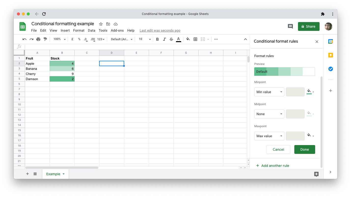
Google Sheets’ implementation is limited, but very easy to use. Select a range of numbers, as before, but this time, change the tab near the top of the Conditional format rules window from Single color to Color scale.

Under Format rules you can define the nature of your color scale. Clicking the Preview button reveals a limited set of predefined palettes to choose from. You can customize the scale by selecting different values or percentages to represent the minimum color point, the maximum color point, and the midpoint. The color pickers alongside each point allow for more control over the color palette.

Other Aspects to Consider

If you make extensive use of this feature in a spreadsheet, it can be easy to lose track of what conditional formatting rules you put in place. The side panel gives no way of viewing all the rules in play; it simply shows which rules are set up for the currently selected cells.

To view all your rules, select all cells using either the keyboard shortcut (Ctrl/Cmd + A) or by clicking the blank rectangle in the very top-left corner before row 1 and column A.

Note that if you copy and paste a cell containing conditional formatting, you’re also copying that conditional formatting for that cell.

Finally, if you create multiple contradicting rules for a cell or range, only the first rule applies. You can change the order by dragging a rule using the vertical dots icon on its left side.

Save Time and Ensure Consistency With Conditional Formatting

Conditional formatting is the kind of Google Sheets feature that can save a lot of time, although you could easily go without ever knowing it exists. Even at the simplest level, it allows you to present spreadsheet data with added meaning, without additional on-going effort.

MakeUseOf – Feed

  • Tweet
Tagged under: Conditional, Formatting, Google, Sheets

About rudy deighton

What you can read next

The Best Dark Web Browser for Your Device
Charge All the Things, With the Mophie Powerstation Hub
5 Tools to Sync & Auto-Upload Photos from Android to Cloud Storage

Rudy Deighton Corporate Blog

  • Your Microsoft Account: 5 Things Every Windows User Should Know

    Your Microsoft account is Microsoft’s sin...
  • Italy Limits Access to TikTok Following a Child’s Death

    Italy is cracking down on TikTok after a 10-yea...
  • Apple Watch Helped Police Find a Kidnapping Victim

    This guide is available to download as a free P...
  • Adobe Photoshop for iPad vs. Affinity Photo for iPad: Which Is Best?

    Adobe Photoshop is the go-to when it comes to i...
  • Microsoft U-Turns Over Xbox Live Gold Price Hike

    Users of Microsoft’s Xbox Live Gold servi...
  • The 10 Best CES Products You Can Buy Right Now

    CES often grabs headlines for its wacky concept...
  • Future Siri Could Recognize How Far Away Your Voice Is

    Since Siri made its debut in 2011 with the iPho...
  • What Is Thread and What Does It Mean for Your Smart Home?

    Included in Apple’s HomePod mini is a new...
  • Pinterest Now Pins "Stories" to the Top of Your Feed

    You didn’t read that wrong. Even Pinteres...
  • Microsoft’s To Do App Now Uses AI to Predict Your Schedule

    If you struggle to draw up a schedule for a giv...
  • Locked Out? How to Reset Your PlayStation Password

    If you’re trying to get into your PlaySta...
  • Looking to Stream Your Nintendo Switch Gameplay? Llano Microdock 3-in-1 Offers Charge, HDMI Out, and Capture

    Llano MicroDock for Nintendo Switch 9.00 / 10 R...
  • Learn How to Become a Better Leader With This Online Course

    It’s not easy to be an effective leader. ...
  • Google Calendar on the Web Gets Offline Support

    We’ve all been there. You’re trying...
  • Report: The Entire iPhone 13 Lineup Will Use Sensor-Shift OIS

    Apple will reportedly bring one of the best pho...
  • Apple’s Next Fitness Challenge Celebrates Black History Month

    Apple’s next fitness challenge will invite Appl...
  • First Wearable Blood-Glucose Tracker Could Save Millions of Lives

    Did a startup invent the holy grail of health w...
  • Joe Biden Invites Everyone to His Inauguration Via Snapchat

    The inaugural committee behind US President-ele...
  • Remember the Banned PS5 Faceplate Seller? It’s Back…

    You may feel like you’re experiencing déj...
  • Microsoft Launches Native Microsoft Edge Beta for M1-Based Macs

    It’s good news for macOS users, as Micros...
  • Parler Is Back Online, But It’s Still Unusable

    After Amazon Web Services dropped Parler for la...
  • How to Sign Out of Netflix on Your Smart TV

    Netflix is available on every device under the ...
  • HBO Max Continues to Offer 20% Off Subscriptions

    If you’ve been thinking of signing up to ...
  • 6 Useful iPhone Group Chat Tips You Should Know

    Engaging in iMessage group conversations can be...
  • How To Protect Yourself From Fraudulent Stores on Shopify

    Shopify, an affordable e-commerce platform used...
  • How to See Who Viewed Your Instagram Posts

    Instagram has been the internet’s favorit...
  • How to Edit Videos on Windows 10

    Editing videos on a Windows PC isn’t as difficu...
  • What Is Facebook’s Collab App and How Do You Use It?

    If you want to do more than scroll through your...
  • GUI? What Is a Graphic User Interface?

    GUIs are ubiquitous, yet you may not even know ...
  • How to Change the Background Color on an Instagram Story

    Looking for a way to personalize your Instagram...
  • How to Secure Freelance Work on Reedsy’s Marketplace

    How to Secure Freelance Work on Reedsy’s ...
  • iMac Is Due To Receive Its First Design Upgrade Since 2012

    It’s a testament to the iMac that, despit...
  • WhatsApp Delays New Privacy Policy After Facebook Data Sharing Controversy

    WhatsApp is now delaying the implementation of ...
  • The 7 Best Gaming Chairs in 2021

    Summary List 8.20/10 1. Premium pick: Vertagear...
  • Epic Games Files New Legal Complaint Against Apple

    The battle between Apple and Fortnite-maker Epi...
  • Google Officially Owns Fitbit: What That Means For You

    Google took to The Keyword to announce that its...
  • Samsung’s New Galaxy SmartTag Has Some Serious Shortcomings

    Samsung has entered into the tracking device se...
  • Oculus Quest to Get Account Sharing Features

    Want to share your Oculus Quest or Quest 2 with...
  • ASUS Updates Dual-Screen ZenBook Duo’s With New Intel CPUs

    2020 was the year of the dual-screen smartphone...
  • Report: 2020 Was an Astonishingly Great Year for the App Store

    Apple customers contributed to a mind-boggling ...

DELTA MEDIA ONLINE MARKETING PLATFORM
An Arte di Riunire Investments GmbH Division

Office:
Delta Media

Arte di Riunire Investments GmbH

Address: Lood 207F

Postcode: 3803 Beatenberg (Swiss)

email: rudydeighton@hotmail.com

rudydeighton@deltamediagbe.com


Online Platform

Menu POS Systeem

  • GET SOCIAL
Rudy Deighton

© 2014 Delta Media - Arte di Riunire Investments GmbH Division - SWISS All Rights Reserved

TOP